Custom fitting example

This is a short example for fitting data, which is not covered by the fitting widget. It relies on calling lmfit manually. Therefore one needs to provide a fitting function, which calculates the numerical residual between measurement and model. This notebook is about fitting multiple datasets from different angles of incidents simultaneously, but can be adapted to a wide range of different use cases.

import numpy as np
import elli
from elli.fitting import ParamsHist
from lmfit import minimize, fit_report
import matplotlib.pyplot as plt

Data import

Read Ψ (psi) and Δ (delta) ellipsometric spectra for different angles from a NeXus file, limited to a wavelength range of 210–800 nm, to be compatible with a tabulated Silicon dispersion.

data = elli.read_nexus_psi_delta("SiO2onSi.ellips.nxs").loc[
    (slice(None), slice(210, 800)), :
]
lbda = data.loc[50].index.get_level_values("Wavelength").to_numpy()
data

		Ψ	Δ
Angle of Incidence	Wavelength
50	210.0	40.028156	146.370560
	211.0	40.012478	146.607407
	212.0	40.007420	146.799438
	213.0	40.005928	147.055832
	214.0	40.001190	147.294281
...	...	...	...
70	796.0	9.051100	174.423874
	797.0	9.054414	174.494553
	798.0	9.044289	174.405136
	799.0	9.048944	174.376541
	800.0	9.021362	174.418228

1773 rows × 2 columns

Setting up invariant materials and fitting parameters

Set up the optical constants for the substrate from RII and define initial fit parameters for the Cauchy SiO₂ layer.

rii_db = elli.db.RII()
Si = rii_db.get_mat("Si", "Aspnes")

params = ParamsHist()
params.add("SiO2_n0", value=1.452, min=-100, max=100, vary=True)
params.add("SiO2_n1", value=36.0, min=-40000, max=40000, vary=True)
params.add("SiO2_n2", value=0, min=-40000, max=40000, vary=False)
params.add("SiO2_k0", value=0, min=-100, max=100, vary=False)
params.add("SiO2_k1", value=0, min=-40000, max=40000, vary=False)
params.add("SiO2_k2", value=0, min=-40000, max=40000, vary=False)
params.add("SiO2_d", value=20, min=0, max=40000, vary=True)

Model helper function

This model function is not strictly needed, but simplifies the fit function, as the model only needs to be defined once.

def model(lbda, angle, params):
    SiO2 = elli.Cauchy(
        params["SiO2_n0"],
        params["SiO2_n1"],
        params["SiO2_n2"],
        params["SiO2_k0"],
        params["SiO2_k1"],
        params["SiO2_k2"],
    ).get_mat()

    structure = elli.Structure(
        elli.AIR,
        [elli.Layer(SiO2, params["SiO2_d"])],
        Si,
    )

    return structure.evaluate(lbda, angle, solver=elli.Solver2x2)

Defining the fit function

The fit function follows the protocol defined by the lmfit package and needs the parameters dictionary as first argument. It has to return a residual value, which will be minimized. Here psi and delta are used across all angles to calculate the residual, but could be changed to any other measured quantity like transmission or reflection data.

def fit_function(params, lbda, data):
    residual = []

    for phi_i in [50, 60, 70]:
        model_result = model(lbda, phi_i, params)

        resid_psi = data.loc[(phi_i, "Ψ")].to_numpy() - model_result.psi
        resid_delta = data.loc[(phi_i, "Δ")].to_numpy() - model_result.delta

        residual.append(resid_psi)
        residual.append(resid_delta)

    return np.concatenate(residual)

Running the fit

The fitting is performed by calling the minimize function with the fit_function and the needed arguments. It is possible to change the underlying algorithm by providing the method kwarg. The fit_report function provides fitted values, uncertainties, and goodness-of-fit statistics.

out = minimize(fit_function, params, args=(lbda, data), method="leastsq")
print(fit_report(out))

[[Fit Statistics]]
    # fitting method   = leastsq
    # function evals   = 119
    # data points      = 3546
    # variables        = 3
    chi-square         = 157.748841
    reduced chi-square = 0.04452409
    Akaike info crit   = -11031.1779
    Bayesian info crit = -11012.6572
[[Variables]]
    SiO2_n0:  1.63549687 +/- 0.03012997 (1.84%) (init = 1.452)
    SiO2_n1:  27.6408771 +/- 8.75248298 (31.66%) (init = 36)
    SiO2_n2:  0 (fixed)
    SiO2_k0:  0 (fixed)
    SiO2_k1:  0 (fixed)
    SiO2_k2:  0 (fixed)
    SiO2_d:   1.75831329 +/- 0.02404272 (1.37%) (init = 20)
[[Correlations]] (unreported correlations are < 0.100)
    C(SiO2_n0, SiO2_d)  = -0.9916
    C(SiO2_n0, SiO2_n1) = -0.9596
    C(SiO2_n1, SiO2_d)  = +0.9259

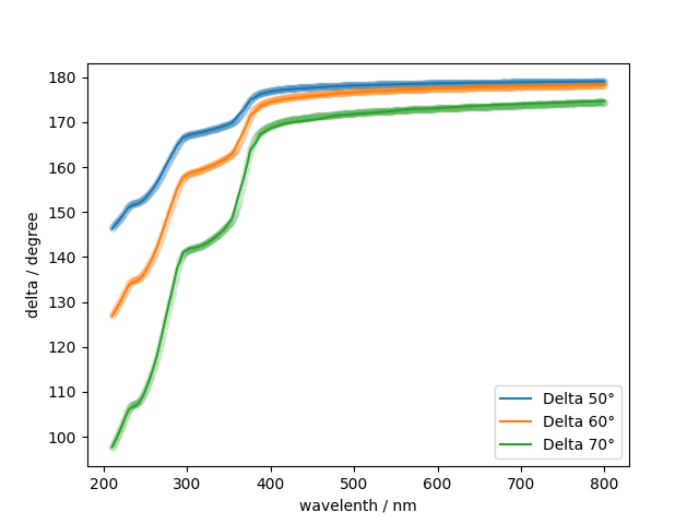
Plotting the results

The measurent results are displayed as scatter plot and the PyElli results are overlayed as solid lines.

fit_50 = model(lbda, 50, out.params)
fit_60 = model(lbda, 60, out.params)
fit_70 = model(lbda, 70, out.params)

fig = plt.figure(dpi=100)
ax = fig.add_subplot(1, 1, 1)
ax.scatter(lbda, data.loc[(50, "Ψ")], s=20, alpha=0.1, label="50° Measurement")
ax.scatter(lbda, data.loc[(60, "Ψ")], s=20, alpha=0.1, label="Psi 60° Measurement")
ax.scatter(lbda, data.loc[(70, "Ψ")], s=20, alpha=0.1, label="Psi 70° Measurement")
(psi50,) = ax.plot(lbda, fit_50.psi, c="tab:blue", label="Psi 50°")
(psi60,) = ax.plot(lbda, fit_60.psi, c="tab:orange", label="Psi 60°")
(psi70,) = ax.plot(lbda, fit_70.psi, c="tab:green", label="Psi 70°")
ax.set_xlabel("wavelenth / nm")
ax.set_ylabel("psi / degree")
ax.legend(handles=[psi50, psi60, psi70], loc="lower left")
fig.canvas.draw()

fig = plt.figure(dpi=100)
ax = fig.add_subplot(1, 1, 1)
ax.scatter(lbda, data.loc[(50, "Δ")], s=20, alpha=0.1, label="Delta 50° Measurement")
ax.scatter(lbda, data.loc[(60, "Δ")], s=20, alpha=0.1, label="Delta 60° Measurement")
ax.scatter(lbda, data.loc[(70, "Δ")], s=20, alpha=0.1, label="Delta 70° Measurement")
(delta50,) = ax.plot(lbda, fit_50.delta, c="tab:blue", label="Delta 50°")
(delta60,) = ax.plot(lbda, fit_60.delta, c="tab:orange", label="Delta 60°")
(delta70,) = ax.plot(lbda, fit_70.delta, c="tab:green", label="Delta 70°")
ax.set_xlabel("wavelenth / nm")
ax.set_ylabel("delta / degree")
ax.legend(handles=[delta50, delta60, delta70], loc="lower right")
fig.canvas.draw()

• 
•